Generating tabular data with a GAN, one tiny network per row

GANs were producing faces nobody could tell from photos, and a collaborator and I wanted to know whether the same idea could produce rows of a spreadsheet. We worked on it through spring 2022. The code and poster are on GitHub at despresj/ece_colab.

The idea came from a statistics question more than a deep learning one. Randomized controlled trials are expensive, and sample size limits how confident you can be in an estimate. Could a GAN learn a trial dataset well enough to generate extra synthetic patients that make a model or test stronger? Privacy was a second motivation: convincing synthetic rows could be shared where the originals can’t. The plan was to generate rows, check them with plots and tables, train a model on them, and see whether it matched a model trained on the real data.

The short version: we got a GAN to produce plausible-looking taxi trips by training many tiny networks and filtering the output. It learned where taxis are, but not how trips connect places.

The stroke data

We started with the International Stroke Trial, a public research dataset described in Sandercock et al. (2011, doi:10.1186/1745-6215-12-101). It has 19,435 patients from 36 countries who were randomized to aspirin or no aspirin, and separately to heparin or no heparin. The file has 112 columns: baseline symptoms and vitals, what was given in the first 14 days, and outcomes at 14 days and six months. I computed the outcome balance from the raw file:

Outcome	Patients	Share
Dead at 14 days	2,034	10.5%
Dead by six months	4,370	22.5%
Alive at six months	15,065	77.5%

Six-month deaths use the dataset’s DIED indicator. It agrees with the six-month follow-up death flag in all but one row.

Death by six months was the obvious target, and the classes are unbalanced. A model that predicts “survived” for everyone is right 77.5% of the time, so that’s the bar.

The first GAN

A GAN is two networks trained against each other. The generator turns random noise into a row of data, and the discriminator outputs the probability that a row is real.

We started on the stroke data. With the columns standardized, a small demonstration on five of them behaved the way a GAN is supposed to:

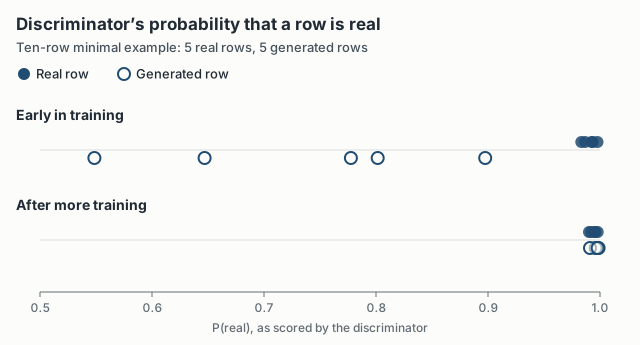
Early on, the discriminator is sure the real rows are real (0.98 and up) and doubtful about the generated ones (0.55 to 0.90). After more training it gives every row 0.99 or higher and can’t tell them apart. This is ten rows, and a fooled discriminator is not evidence that the rows are useful. It at least showed the training loop doing what it should.

Taxi trips

The problem with the stroke data was checking the output. If a GAN produces an elderly patient with high blood pressure and a particular pattern of deficits, there’s no easy way to say whether that patient is plausible. We needed data where a bad row is obviously bad.

So we switched to New York City taxi trips from 2016: 1,458,644 trips, each with pickup and drop-off times and coordinates, passenger count, and trip duration. I split each timestamp into calendar features (month, day, hour, day of week, and so on), which gave 28 columns, and scaled everything to between 0 and 1. A generated ride in the 14th month, on day −5, or ending in a river is easy to spot and filter.

The main problem was mode collapse. A trained generator would settle on a handful of outputs and produce them no matter what noise went in. Our workaround was blunt: train a new, very small GAN for every batch of output, with a randomly drawn architecture (8 to 24 neurons per layer, a random number of layers, random learning rates), and keep one row from each round of training. It worked, in the sense that the output varied. It was also slow. The training log shows 1,020 of 5,000 runs finishing in 7 hours 36 minutes, about 27 seconds per run, and a full batch took 18 to 24 hours on a Colab P100 GPU. Most of what came out had to be thrown away.

What came out

After filtering, most generated rides were plausible. But they didn’t have the same structure as the real data. The real trips include a lot of rides from the airports into Midtown. The generated trips mostly started in Midtown and went to other parts of Midtown or out to the surrounding boroughs, and a few ended in rivers or on expressways. The GAN learned where taxis usually are. It didn’t learn how trips connect places.

Tabular data isn’t a small image. Its columns mix scales and types, and whether a row is plausible depends on relationships between columns, like a drop-off coming after its pickup. “Looks plausible” also isn’t a metric. Checking by eye only worked because we picked data you can put on a map, and clinical trial data can’t be checked that way.

At a day of GPU time per batch, an approach like this has to beat something cheap, like bootstrapping or a simple parametric model, to be worth it.