Testing 20,000 SNPs at once

When you test 19,996 SNPs for an association with one phenotype, how do you decide which results to believe? The data set had genotypes for 10,000 people at 19,996 SNPs (single-letter positions in the genome where people differ), plus one numeric phenotype for each person, and I tested every SNP.

The statistics in each test are easy. The hard part is that there are 19,996 of them.

One regression per SNP

For each SNP j, fit a simple linear model:

y = μ + x_j · b_j + error

where x_j is the genotype coded 0, 1, or 2 (the number of copies of one allele), and test whether b_j is zero. That gives one p-value per SNP.

I wrote it the obvious way: a for loop over the columns, lm(y ~ X[, i]) each time, pulling the slope’s p-value out of summary(). With 10,000 rows that is 19,996 model fits. It worked, but slowly enough that I put a progress bar on it and cached the chunk so I wouldn’t have to rerun it every time I knitted the document.

There’s a faster route I didn’t use at the time. For a simple regression with one predictor, the t-test on the slope is the same test as the t-test on the Pearson correlation between x_j and y. You can compute all 19,996 correlations with one matrix product, turn each into a t-statistic with t = r · √((n − 2) / (1 − r²)), and get the p-values from pt(). When I checked this against lm() on a few columns, the p-values agreed to about 12 significant digits.

Why you can’t just use 0.05

If none of the SNPs had any effect, a 0.05 cutoff would still flag about 5% of them, or roughly 1,000 SNPs, by chance alone. So I used three standard adjustments, all available through p.adjust() in R.

Bonferroni rejects when p < 0.05 / m, where m is the number of tests. Here that’s 0.05 / 19,996 ≈ 2.5 × 10⁻⁶, or about 5.6 on the −log10 scale. It controls the family-wise error rate, the chance of making even one false discovery. It is simple and very strict.

Holm sorts the p-values from smallest to largest, compares the smallest to 0.05 / m, the next to 0.05 / (m − 1), and so on, and stops at the first one that fails. It has the same family-wise guarantee as Bonferroni and never rejects less. But when only a handful of SNPs are real, the thresholds for the first few steps are nearly identical, so in practice it usually rejects the same set.

Benjamini–Hochberg (BH) also sorts the p-values, then finds the largest rank k where p_(k) ≤ k · 0.05 / m and rejects everything up to that rank. This controls the false discovery rate: among the SNPs you call significant, the expected share of false ones is at most 5%. It accepts a few false positives in exchange for finding more real ones.

Bonferroni and Holm answer “how sure am I that none of these are flukes?” BH answers “what fraction of this list do I expect to be flukes?” For a first-pass genome scan whose results get followed up, the second question is often the more useful one.

Three plots of the raw p-values

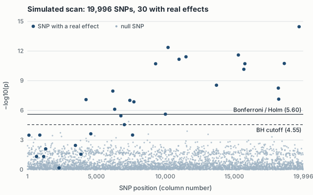
I also made three pictures of the unadjusted p-values. A Manhattan plot puts −log10(p) against SNP position, and real signals stick up above the background. A histogram of the p-values with 500 bins should be flat under the null, with any real signal showing up as a spike near zero. A QQ plot on the −log10 scale puts the observed p-value quantiles against the quantiles expected from a uniform distribution, with a 45-degree line for reference.

The QQ plot is where you can see the scan clearly depart from the null. My read on the real data was that the points start bending away from the line at around 2.5 on the −log10 scale, which is a p-value of roughly 0.003.

A simulation with the same shape

The original data set isn’t public, and I no longer have a copy, so I can’t reproduce the list of significant SNPs I found. To show how the three methods behave, I ran a simulation with the same shape: 10,000 people and 19,996 SNPs. Thirty of the SNPs have a real effect, each explaining between 0.05% and 0.5% of the phenotype’s variance. Everything below comes from that simulation, not the original data.

Method (simulated data)	SNPs flagged	Real	False
Unadjusted p < 0.05	1,001	29	972
Bonferroni	18	18	0
Holm	18	18	0
Benjamini–Hochberg	21	20	1

Unadjusted testing is useless at this scale. It catches 29 of the 30 real SNPs, but they’re buried among 972 false ones. Holm matched Bonferroni exactly, which is the usual outcome when the true signals are sparse. BH found two more real SNPs and let in one false one. Its cutoff landed at p ≈ 2.8 × 10⁻⁵ (4.55 on the −log10 scale), about ten times looser than Bonferroni’s, and one false discovery out of 21 is within what a 5% false discovery rate allows.

Ten real SNPs were missed by every method. Their effects were too small to separate from noise with 10,000 people, and the strongest of them only reached about 3.6 on the −log10 scale. Correcting for multiple tests costs power, and no choice of adjustment gets that power back.

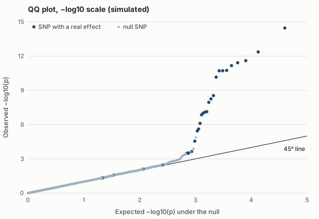
The QQ plot shows the same picture from a different angle. The bulk of the SNPs sits on the line, and the handful of real ones pull the upper tail away from it. In this simulation the bend starts somewhere between 2.5 and 3.

Toward a real scan

On a scan this size, the correlation shortcut is worth using: it replaces 19,996 model fits with a single matrix product.

The model itself would need more for a real scan. Neighboring SNPs are inherited together (linkage disequilibrium), so one real signal usually shows up as a tower of nearby hits. That correlation also makes Bonferroni more conservative than it needs to be. My simulation draws every SNP independently, so it doesn’t capture any of this.

A real association scan would also include covariates such as ancestry, because population structure alone can produce apparent associations. My model had none, which was fine for learning the multiple-testing part but not for anything beyond that.