Simulating power for a BMI and blood pressure regression

If you want to measure how body mass index affects systolic blood pressure, how many people do you need to recruit? It’s a standard question, and I answered it without a power formula, by simulation.

The setup

The research goal was to estimate the effect of BMI on systolic blood pressure (SBP) while accounting for sex. The model was:

SBP ~ BMI + Sex

Every part of the simulated world was fixed in advance:

• Half the sample is male, half female.
• BMI for women is normal with mean 26.5 and variance 30. For men, mean 27.4 and variance 16.7.
• SBP = 120 − 3·Male + b2·Z + error, where Z is BMI centered on the sample mean and the error variance is 300.
• Fit the model with lm() and reject when the p-value on centered BMI is below 0.05.

Power is the share of simulated studies that reject. For each total sample size N (30, 50, 100, 200, 500, 1,000 and 3,000) and each effect size b2 (0, 0.2, 0.3 and 0.5 mmHg per BMI point), I generated a fresh dataset, fit the model, recorded whether the BMI coefficient was significant, and repeated that 10,000 times.

Where the numbers come from

The numbers below come from running the simulation exactly as specified above, with seed 55555 and 10,000 replicates per cell.

To make that fast, I replaced lm() with the closed-form equivalent. With a single binary covariate, the t-test on the BMI slope is the same as regressing within-sex-centered SBP on within-sex-centered BMI, with n − 3 degrees of freedom. On a few hundred test datasets, those p-values matched summary(lm()) to about 1e-15. With the replacement, 280,000 model fits took seconds.

Power curves

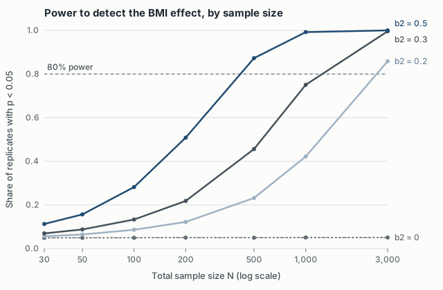
N	b2 = 0.2	b2 = 0.3	b2 = 0.5
30	0.057	0.070	0.113
100	0.086	0.133	0.282
200	0.122	0.218	0.509
500	0.232	0.456	0.873
1,000	0.422	0.751	0.992
3,000	0.859	0.996	1.000

The b2 = 0 runs, which I left out of the table, work as a check, and it’s the cheapest one there is. When there is no effect, the rejection rate should equal the Type I error rate, and it does: every cell falls between 0.0488 and 0.0509. With 10,000 replicates, the Monte Carlo standard error at 0.05 is about 0.002, so those values are consistent with 0.05.

The other columns show the usual pattern. What drives power is the effect size times the square root of N. A BMI effect of 0.5 is detectable with a few hundred people. An effect of 0.2 needs thousands. At N = 30, even the largest effect is detected only about 11% of the time.

How many people for 80% power at b2 = 0.3?

The coarse grid put the answer between 1,000 (0.751) and 3,000 (0.996). To narrow it, I ran the same simulation at every even N from 1,100 to 1,200, again with 10,000 replicates each.

Here the simulation noise starts to matter. With 10,000 replicates, the standard error of a power estimate near 0.8 is about 0.004. Neighboring sample sizes differ by far less than that in true power, so the estimated curve jitters. The first N with an estimate at or above 0.80 was 1,124 (0.805). But N = 1,140 dipped back to 0.798. Taking the first point that crosses the line mostly measures luck.

Fitting a straight line through the 51 grid points and solving for 0.80 gave N ≈ 1,127. As a sanity check, the normal-approximation formula with a pooled within-sex BMI variance of 23.35 gives about 1,120. So the answer is around 1,120 to 1,130 people, and I’d plan for a bit more.

A while loop that increases N until the estimated power first passes 0.8 has the same weakness as reading the first crossing off the grid, since it’s a noisy stopping rule. Fitting a line through the grid gives a steadier answer.

Interaction effects

A harder version of the question: suppose BMI raises blood pressure by 0.4 per point in men but only 0.2 in women. How large does the study need to be to detect that difference? The model adds a sex × BMI interaction, and the test is on the interaction coefficient, which is 0.2 here. The rest of the setup is unchanged, and the sample size goes up to 10,000.

N	Power to detect the interaction
500	0.091
1,000	0.128
3,000	0.312
5,000	0.475
10,000	0.762

Even at 10,000 people, the power is only 0.76. The normal approximation puts 80% power at roughly 11,000. The reason is that an interaction is a difference between two slopes, each estimated from half the sample. The variance of that difference is much larger than the variance of a single pooled slope, so a study sized for the main effect is badly underpowered for a sex difference of the same magnitude.

When there’s no formula

With a closed-form power formula available, simulating power for a linear model is mostly an exercise. The same loop still works when the formula isn’t available: unequal variances, clustered designs, missing data, odd estimators. The checks carry over unchanged. Confirm the null case rejects about 5% of the time, report the Monte Carlo error, and fit a line through the grid instead of taking the first noisy crossing of 0.8.