Scoring simple forecasts across S&P 500 stocks

Most examples in Hyndman and Athanasopoulos’s Forecasting: Principles and Practice forecast one series and show you one plot, and one plot can’t tell you whether a method is any good. While working through the book, I wanted to run the same basic methods on hundreds of series and look at how the errors were distributed.

Stock prices were a convenient test set: one file of daily closing prices for the companies in the S&P 500. The point was to practice the evaluation workflow. I wasn’t looking for a trading edge, and nothing here should be read as investment advice.

Setup

The data was a long table with one row per ticker per day. I split it by ticker with purrr, turned each ticker’s closing prices into a ts object, and made a matching training set with the last 20 closes removed. Those 20 days were the test set.

A single function, crystal_ball(), took one training series and one full series. It fit four forecasts with a 20-step horizon using the forecast package. The mean method forecasts every future value as the average of the training data, and the naive method forecasts every future value as the last observed price. Holt is exponential smoothing with a linear trend, and damped Holt is the same with the trend flattening out over the horizon. The function scored each forecast against the 20 held-out prices with accuracy() and returned a small table with one row per method.

map2() ran that function over every ticker, and bind_rows() stacked the results into one table with a row for each stock and method.

The metrics

Here’s what accuracy() computes. With actual price y_t, forecast ŷ_t, error e_t = y_t − ŷ_t, and N test points:

• RMSE = √( Σ e_t² / N ). Typical error size, in dollars. Big misses count extra.
• MAE = Σ |e_t| / N. Average absolute miss, in dollars.
• MPE = (100% / N) · Σ e_t / y_t. Average signed percentage error. Positive and negative errors cancel, so it measures bias and can’t tell you how accurate a method is.
• MASE = MAE on the test set ÷ in-sample MAE of a naive benchmark. A value below 1 means the method beat the benchmark’s typical in-sample error.

Errors by method

I summarized the per-stock mean percentage error for each method. The numbers come from the August 2020 run of the analysis.

Method	Median MPE	Mean MPE	Std. dev.
Naive	−1.34%	−2.06%	5.10
Holt	−1.61%	−2.35%	5.14
Holt, damped	−1.28%	−2.00%	5.03
Mean	8.89%	3.87%	24.91

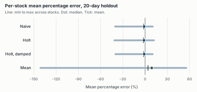
Naive, Holt, and damped Holt were practically the same method here. Their medians were within a third of a percentage point of each other, and their ranges across stocks were almost identical, from about −40% at the low end to 10 to 12% at the high end. Holt’s fitted trend added nothing over “tomorrow’s price equals today’s,” which is about what you’d expect if daily prices behave roughly like a random walk.

The mean method was badly wrong. Stock prices drift over time, so the long-run average of a price series usually sits far from where it currently trades. Its per-stock MPE ranged from −141% to 56%, and its standard deviation was about five times the others’.

The signs say more about the market than about the methods. Errors are actual minus forecast, so a negative MPE means the forecast came in above the realized price. For the naive method, that means the typical stock closed a little below its last training price during the 20 test days. Every stock shared those same 20 days, so all of these errors come from a single draw of market conditions, and the hundreds of stocks don’t add up to hundreds of independent tests.

What I’d try next

MPE shows which way the misses lean, but positive and negative errors cancel, so it says little about how big they are. MAPE or MASE would summarize the size of the misses, and accuracy() already returns MASE for every stock.

The test window matters more than the metric. With a single 20-day holdout, one market move dominates everything. Rolling-origin evaluation, where you refit and forecast from many cutoff dates (tsCV() in the same package), would say much more about how the methods compare.

The baselines won, and that’s the useful result. Before trying anything more elaborate on price data, the naive forecast is the thing to beat, and here the textbook’s more elaborate methods didn’t beat it.