Forecasting frozen veggie burgers, and losing to the naive method
Forecasting weekly Morning Star Farms sales at Walmart and Meijer with fpp2 methods, where the simplest forecast won.
Given a couple of years of weekly unit sales for each product in a grocery line, which standard method best predicts the next few months? We asked that of weekly scanner data for Morning Star Farms, the plant-based frozen food line: veggie burgers, sausage patties, chik’n nuggets, corn dogs, and so on. It was a three-person project in spring 2020, built entirely in R and written up in a reproducible format.
The data
The data covered 104 weeks, from February 2018 to February 2020, at three market levels: Walmart, Meijer, and a total U.S. food roll-up. Each row was one product at one market in one week, with dollar sales, unit sales, and base units. We joined it with a price list and a product category file by UPC. After a lot of string cleanup on product names (trademark symbols, stray ampersands, inconsistent spacing), each product-by-market combination became one weekly time series of base units.
Not every series was usable. Some products only had data for part of the two years, and others were incomplete in ways that would break a forecast. We wrote a small script that plotted every product at every market, then went through the plots and made a list of which to drop. What survived was 44 series. Dropping incomplete series by looking at plots is defensible, but it’s a judgment call. An explicit threshold, something like “at least N weeks with no gaps,” would make it reproducible.
The method
We followed Hyndman and Athanasopoulos’s Forecasting: Principles and Practice (the second edition, which goes with the fpp2 R package). Most of the work was getting 44 series into a shape the forecast functions would accept, and purrr made that manageable. Split the data frame by product, pull out the base-units column, and turn each one into a weekly ts object:
meijer_list_of_lists <- df %>%
  filter(retailer == "Meijer") %>%
  filter(item_description %!in% meijer_bad_plots) %>%
  split(.$item_description) %>%
  map(list("base_units")) %>%
  map(~ts(., start = 1, frequency = 52))
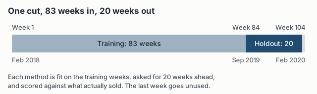
To measure accuracy, we needed forecasts we could check. We cut every series at week 83 (about 80% of the data), fit each method on the first 83 weeks, forecast 20 weeks ahead, and compared the forecast to what sold.
We compared four methods. The mean method forecasts every future week as the average of the training data, and the naive method forecasts every future week as the last observed value. Holt’s linear trend is exponential smoothing with a trend term, and damped Holt is the same, but the trend flattens out over the horizon.
We scored them with RMSE, MAE, mean percentage error (MPE), and mean absolute scaled error (MASE). One function, which we called crystal_ball, ran all four methods on a training series and returned a tidy table of accuracy measures. map2 ran it over every pair of training series and full series, and bind_rows stacked the results for all three markets into one table.
performance_walmart <- map2(training_walmart, walmart_list_of_lists, crystal_ball) %>%
  bind_rows(.id = "id")
Once the pipeline existed, adding a method meant adding a few lines to one function, and it would run across every product at every market.
The result
The naive method won.
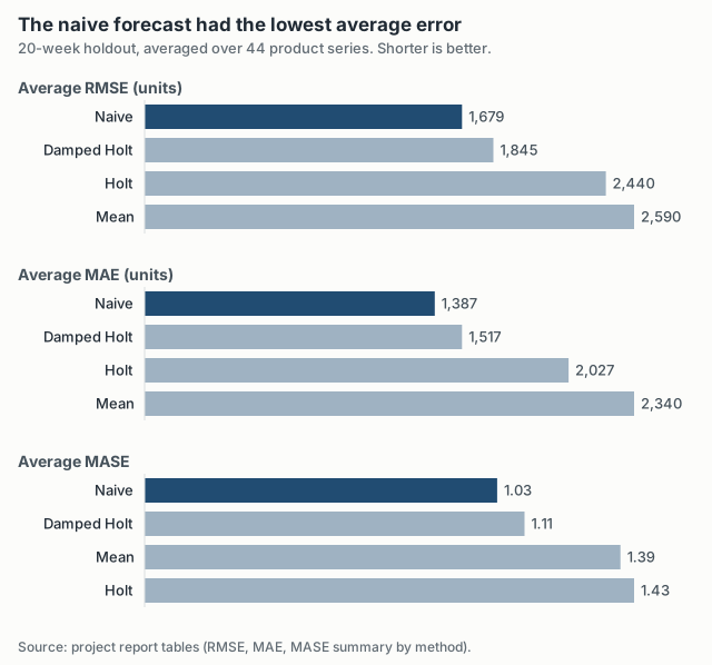
Averaged over the 44 series, the naive forecast’s RMSE was about 9% lower than damped Holt’s and about 35% lower than the mean method’s. On MAE the gap to damped Holt was about the same, around 9%. Damped Holt was a close second on every measure. Undamped Holt did badly: on MASE it came last, behind even the flat mean forecast. It picked up short-term wiggles in the training data as a trend and carried them 20 weeks forward.
The percentage error measures bias, which way the misses lean, and says nothing about their size. In the forecast package, error is actual minus forecast, so a negative MPE means the method forecast too high on average.
| Method | Avg MPE | Median MPE |
|---|---|---|
| Naive | 0.06% | 2.58% |
| Damped Holt | −0.18% | 3.12% |
| Holt | 1.43% | 4.99% |
| Mean | −3.54% | −2.12% |
On the average, naive was almost unbiased. The medians look a little different. For a typical series, naive, Holt, and damped Holt all forecast a few percent low, which is what you’d expect if sales were drifting up a little during the holdout. The mean method’s median bias was actually the smallest in absolute terms, so naive won on the averages but not on every column.
The average MASE for naive, 1.03, also hides a wide spread. The median was 0.49 and the worst series was 8.43, so a handful of series where something changed after the cut pulled the average up. Because the products sell at very different volumes, the averages and medians are the useful summaries, and scale-free MASE is the fairest comparison across products.
Why the naive method won
I don’t think this means the simple method is always best. I think it says something about these series and this setup.
Most of these series looked fairly stable week to week in our plots, and 20 weeks isn’t a long horizon for a product line that isn’t changing quickly. If next week looks like this week, the last observation is hard to beat. The mean method loses because it gives the same weight to weeks from early 2018 as to last week. Holt loses because it finds trends in noise. Damping the trend fixed most of that, which is why damped Holt came close.
It’s also a known result. Hyndman and Athanasopoulos use the naive and mean methods as benchmarks because they are surprisingly hard to beat. We went in expecting the fancier methods to win, and that’s what makes the finding worth reporting.
What to test next
The report ends by saying the real output was the infrastructure for testing more complex methods, and I still agree. ETS, ARIMA, and the seasonal naive method are the obvious next benchmarks. With weekly data and a 52-week season, 83 weeks of training covers the annual cycle less than twice, which makes seasonal methods awkward, but they’re still worth comparing.
Every score here also comes from a single training/holdout split. Time-series cross-validation, refitting at many origins, would say whether naive wins consistently or just happened to win for that stretch of late 2019 into early 2020.