A bootstrap band for gout risk, and an exponential MLE three ways

How uncertain is a logistic regression curve? I used the bootstrap to put a confidence band around one, for gout risk as a function of serum urate. Separately, I estimated the rate of an exponential distribution by maximum likelihood, then compared Hessian and bootstrap standard errors and three kinds of confidence interval.

The numbers below come from rerunning the analysis in R. Each part uses its own seed.

A confidence band for gout risk

The data came from a teaching dataset: 400 people, each with a serum urate (SU) measurement and a record of whether they had gout. Thirty of them did. Serum urate ranged from 2.4 to 12.1 mg/dL.

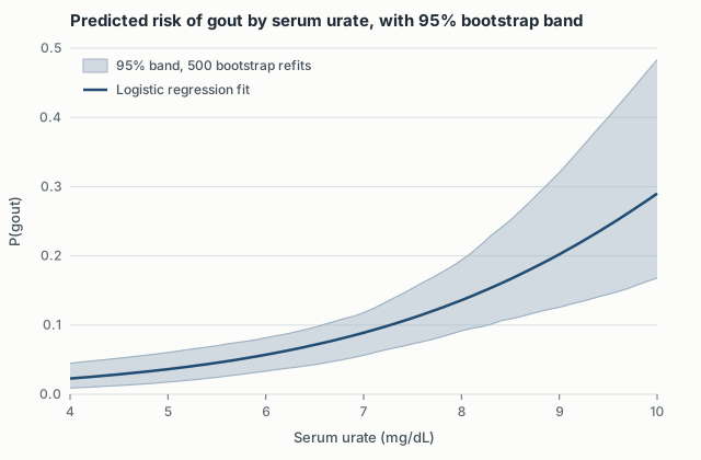
A logistic regression of gout on SU gives a slope of 0.477 per mg/dL (standard error 0.112), an odds ratio of about 1.61 per unit. Converting the fit to predicted probabilities across SU from 4 to 10 gives a smooth curve, and the bootstrap estimates how uncertain it is: resample the 400 people with replacement, refit the model, and predict along the SU grid. Do that 500 times, then take the 2.5th and 97.5th percentiles of the predictions at each SU value.

Serum urate	Predicted risk	95% bootstrap band
4	0.023	0.009 – 0.045
6	0.057	0.033 – 0.082
8	0.136	0.092 – 0.194
10	0.290	0.168 – 0.483

The band widens at high SU because the data thin out: only 17 people had SU above 9. The model gets its confidence at the high end by extending the logistic curve, and the bootstrap shows how much that extension depends on those few people. The band is also asymmetric. It stretches further above the fit than below, which a symmetric plus-or-minus interval would hide.

An exponential MLE three ways

The setup: draw 50 values from an exponential distribution with rate λ = 2 (seed 195021), then estimate λ.

Minimizing the negative log-likelihood with optimize() gave λ̂ = 3.2472. The closed-form MLE is 1/x̄, and x̄ = 0.308, so 1/x̄ = 3.2472. The two agree to about 7e-7. This sample happens to run low: the true mean is 0.5, so λ̂ comes out high.

I got the standard error two ways. The inverse of the numerical Hessian of the negative log-likelihood at λ̂ gives an SE of 0.459, which matches the analytic λ̂/√n. Bootstrapping 10,000 resamples of the 50 values and computing 1/x̄ for each gives an SE of 0.493. The bootstrap SE is about 7% larger. That’s plausible: 1/x̄ is skewed, and the Hessian SE is a local quadratic approximation at the peak.

The confidence intervals:

Method	Lower	Upper
Normal, Hessian SE	2.35	4.15
Normal, bootstrap SE	2.28	4.21
Bootstrap percentile	2.50	4.44

The two normal intervals are symmetric around 3.25. The percentile interval sits to the right, which reflects the right skew of the reciprocal of a mean. None of the three contains the true λ = 2, and no method is at fault for that. This particular sample of 50 is unusually low, and about one sample in twenty should produce an interval that misses.

Is the MLE biased?

The answer depends on keeping the rate and its mean straight. Over 100,000 fresh samples of 50, the average of 1/λ̂ = x̄ was 0.50005, and x̄ is unbiased for the mean 1/λ. The MLE λ̂ = 1/x̄ is not unbiased for λ. Its expected value is nλ/(n − 1). Averaging λ̂ itself over 100,000 samples gives 2.0405, against a theoretical 2.0408 and a true value of 2.0. That’s a 2% upward bias at n = 50, and the simulation’s standard error (0.0009) is small enough to see it clearly.

The bootstrap finds this bias from the single sample. The average of the 10,000 bootstrap λ̂’s was 3.315, which puts the bootstrap bias estimate at +0.067. The theoretical bias at this λ̂, λ̂/(n − 1), is 0.066. The bias is small compared with the SE of about 0.46, so it hardly matters for inference at this sample size. But it exists.